Lots of charts
First things first: I've uploaded a new version with some minor ergonomic improvements for non-mobile devices: some of the menu buttons now have keyboard shortcuts. They were noticeably more difficult to click on with a mouse than on a touchscreen.
There are also tooltips when you hover on the menu buttons which should hopefully make it easy to learn about and remember the keyboard shortcuts.
If you're on a mobile device, nothing should change. No need to upgrade.
To test this new version I've been spending more time running Carousel on my laptop. Today's program is a library for plotting charts in various ways.
I want this for myself, but there's also an element of academic curiosity here. There are various tools for drawing charts: gnuplot, JGraph, Excel. Programming languages like R, Matlab and Python also have common tools. One property all these approaches share* is an ad hoc, accreting set of configuration options. Look at gnuplot's plot, for example. Tutorials tend to be cookbooks for some common uses followed by a link to the manual. Not to be too critical -- I'm never going to match these tools on features -- but I've wondered for a long time if there might be a cleaner set of building blocks that fit my brain better. This is a start, so let's get started. Feel free to follow along by pasting the following code snippets into a screen in Carousel.
* - Matplotlib for Python might be an exception. Its API looks fine at first glance, albeit more verbose. But I haven't actually used it myself yet.
Here's a table with some randomly generated data:
data = {}
-- 16 sample points x 5 units apart = 80
for i=1,16 do
  table.insert(data, {i*5, rand(60), rand(60)})
end
I'm going to ignore for this post the question of how to get data into Carousel. Particularly on mobile. (Not a very clean story. Yet.)
Also, I'm deliberately shaping this data to simplify rendering. A previous post is more flexible in this respect, but we'll not go there today. We'll skip the code for panning and zooming, even if positioning the chart on screen now gets a bit verbose:
-- decide how large a 80:60 image you can fit
H = Safe_height-Menu_bottom
if Safe_width/80 < H/60 then
  -- landscape
  v = {left=50, right=Safe_width-50}
  local h = (v.right-v.left)/80*60
  v.top = Menu_bottom + (H-h)/2
  v.bottom = v.top + h
else
  -- portrait
  v = {top=Menu_bottom+50, bottom=Safe_height-50}
  local w = (v.bottom-v.top)/60*80
  v.left = (Safe_width-w)/2
  v.right = v.left + w
end
-- at this point, 80/(v.right-v.left) == 60/(v.bottom-v.top)
line(v.left, v.top, v.left, v.bottom)
line(v.left, v.bottom, v.right, v.bottom)
Hit 'run' and we finally have some bare axes.
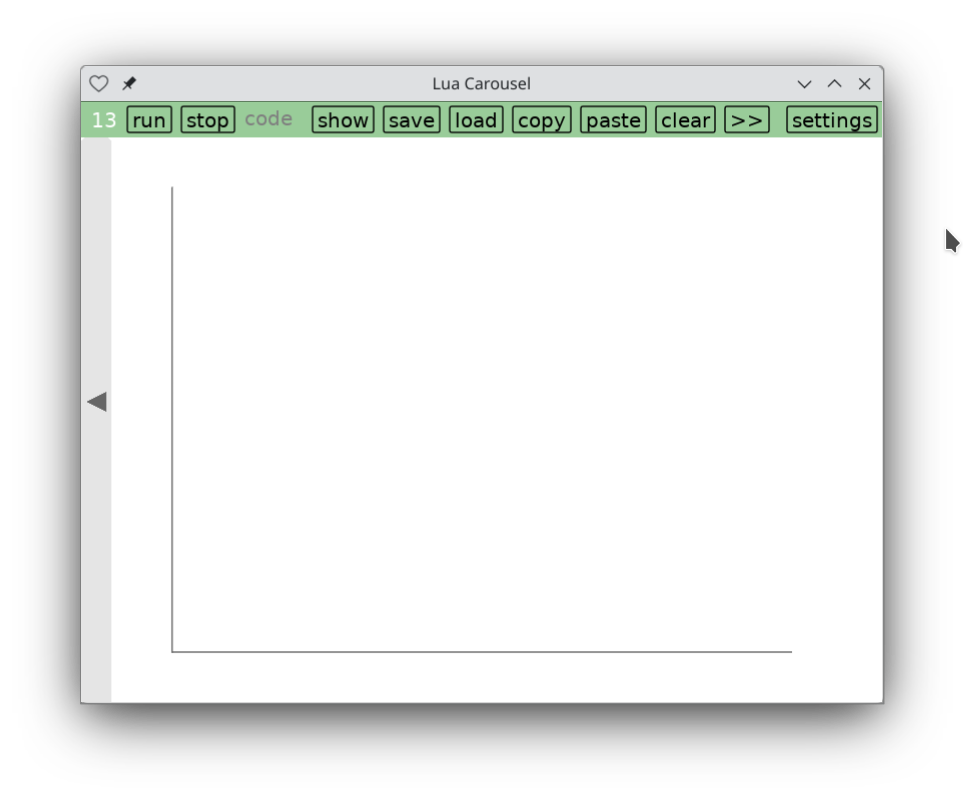
(Won't automatically redraw when rotating the device. Hit 'run' again if you rotate.)
The variable `v` (for 'viewport') now provides a bounding box, and here are a couple of helpers to translate data to within this bounding box:
function vx(x) return v.left + scale(x) end
function vy(y) return v.bottom - scale(y) end
function scale(d) return d/80*(v.right-v.left) end
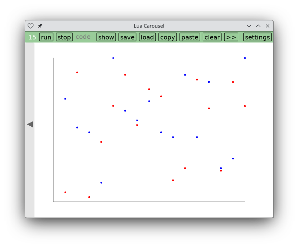
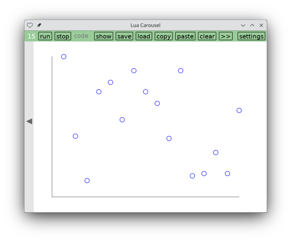
Now we can draw a couple of scatterplots based on `data`:
function col(c)
  return function(data, i) return data[i][c] end
end
function plot(data, f, ...)
  for i=1,#data do f(data, i, ...) end
end
function points(data, i, x, y)
  circle('fill', vx(x(data, i)), vy(y(data, i)), 3)
end
color(1,0,0)
plot(data, points, col(1), col(2))
color(0,0,1)
plot(data, points, col(1), col(3))
Slow down to read the definition of `col`. It's a way to extract columns from the data, but it returns a function that `plot` can call. No special new syntax for columns, just plain Lua. And it's flexible enough to handle data where the rows are key-value tables rather than arrays as above. I can pass a column name rather than a column number to `col`, and it'll just work.
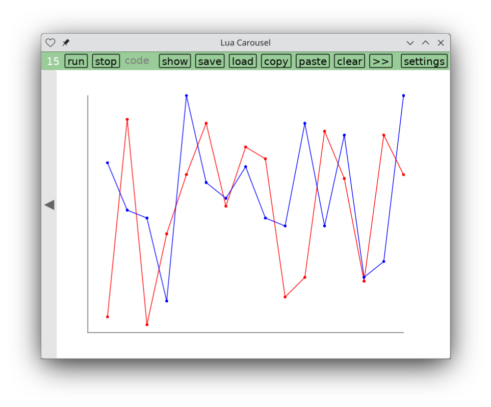
`plot` takes another function as its argument above: `points`, which provides the strategy to follow to plot my data. Here are some other strategies I can swap in (I based their names on the gnuplot manual):
function lines(data, i, x, y)
if i == 1 then return end
line(vx(x(data, i-1)), vy(y(data, i-1)), vx(x(data, i)), vy(y(data, i)))
end
function linespoints(data, i, x, y)
circle('fill', vx(x(data, i)), vy(y(data, i)), 3)
if i == 1 then return end
line(vx(x(data, i-1)), vy(y(data, i-1)), vx(x(data, i)), vy(y(data, i)))
end
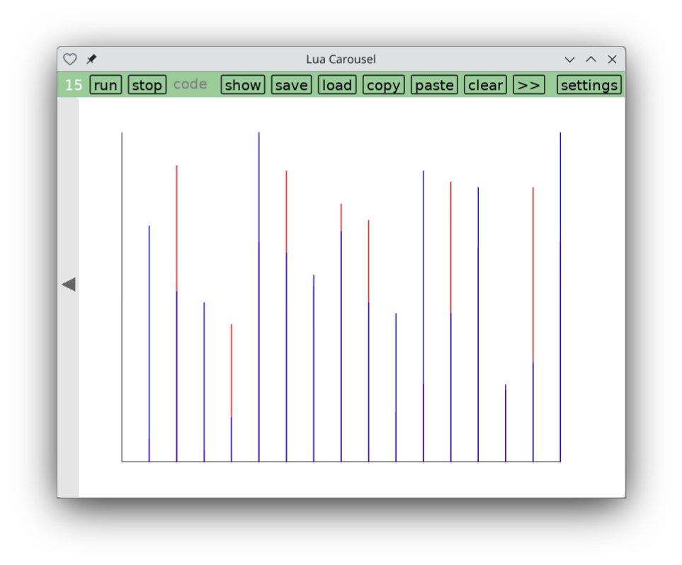
function impulses(data, i, x, y)
local vx = vx(x(data, i))
line(vx, vy(y(data, i)), vx, vy(0))
end
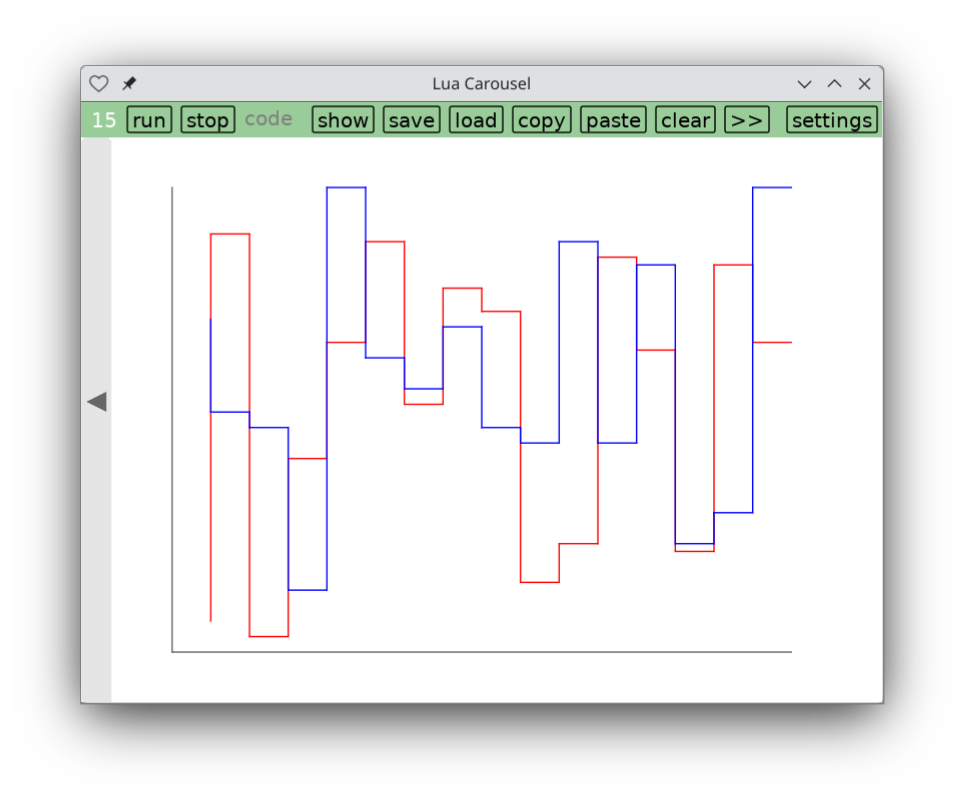
function steps(data, i, x, y)
if i == 1 then return end
local x1, y1 = x(data, i-1), y(data, i-1)
local x2, y2 = x(data, i), y(data, i)
line(vx(x1), vy(y1), vx(x1), vy(y2))
line(vx(x1), vy(y2), vx(x2), vy(y2))
end
function fsteps(data, i, x, y)
if i == 1 then return end
local x1, y1 = x(data, i-1), y(data, i-1)
local x2, y2 = x(data, i), y(data, i)
line(vx(x1), vy(y1), vx(x2), vy(y1))
line(vx(x2), vy(y1), vx(x2), vy(y2))
end
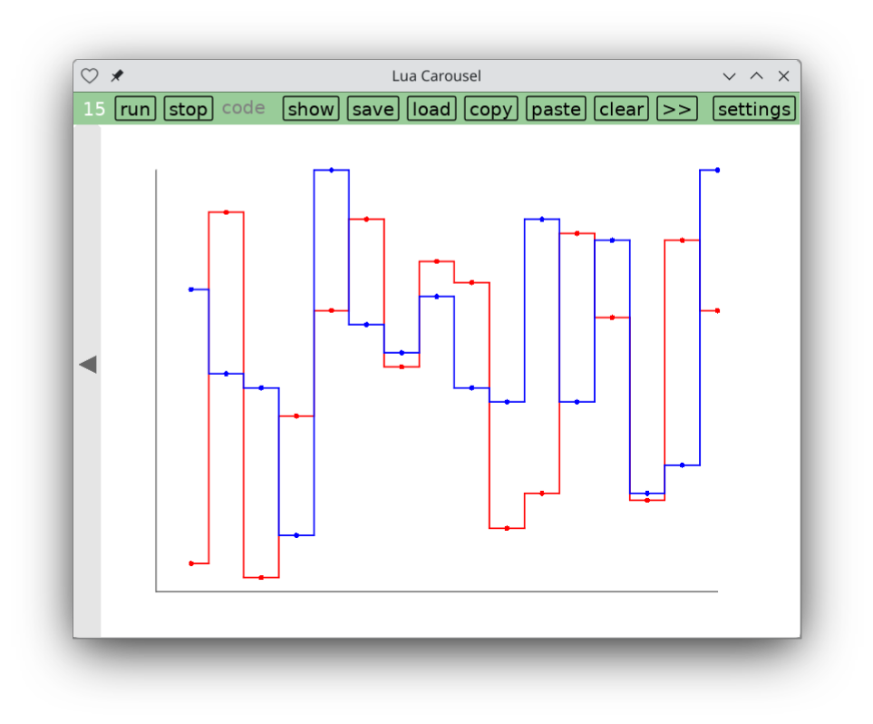
function histeps(data, i, x, y)
local x2, y2 = x(data, i), y(data, i)
circle('fill', vx(x2), vy(y2), 3)
if i > 1 then
local x1, y1 = x(data, i-1), y(data, i-1)
local px, py = (x1+x2)/2, (y1+y2)/2
line(vx(x1), vy(y1), vx(px), vy(y1))
line(vx(px), vy(y1), vx(px), vy(y2))
line(vx(px), vy(y2), vx(x2), vy(y2))
end
if i < #data then
local x3, y3 = x(data, i+1), y(data, i+1)
local nx, ny = (x2+x3)/2, (y2+y3)/2
line(vx(x2), vy(y2), vx(nx), vy(y2))
line(vx(nx), vy(y2), vx(nx), vy(y3))
line(vx(nx), vy(y3), vx(x3), vy(y3))
end
end
Here are the corresponding images for these strategies, all for the exact same data points, and with links to the corresponding gnuplot documentation. Just replace the word 'points' in the calls to `plot` above with:

All the above strategies require two columns of data, for x and y coordinates. But `plot` can handle any number of columns if a strategy needs it. Let's first regenerate a few more columns:
data = {}
for i=1,16 do
  local angle1 = rand(60)/60*pi
  table.insert(data, {i*5, rand(60), rand(60), rand(60)/60*10, rand(60)/60*10, angle1, angle1+rand(60)/60*pi, tostring(rand(1000))})
end
Don't bother reading this. I'm basically generating 2 large numbers, 2 small numbers and 2 angles between 0 and 360 degrees.
Here's a strategy with more arguments, that uses more columns for each object on the chart:
function circles(data, i, x, y, radius, drawmode)
  if type(radius) == 'function' then radius = radius(data, i) end
  circle(optional(drawmode, data, i, 'fill'), vx(x(data, i)), vy(y(data, i)), scale(radius))
end
function optional(f, data, i, default)
  if f == nil then return default end
  if type(f) == 'function' then return f(data, i) end
  return f
end
Now we can draw circles with a fixed radius:
plot(data, circles, col(1), col(2), 1)

Circles with outlines but not filled in, thanks to the `optional` helper above:
plot(data, circles, col(1), col(2), 1, 'line')
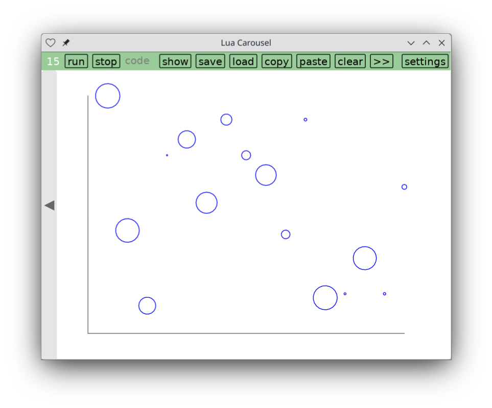
Circles with a radius based on column 4:
plot(data, circles, col(1), col(2), col(4), 'line')
More strategies:
function boxes(data, i, x, y, w)
  local w = optional(w, data, i, 5)
  local y = y(data, i)
  rect('fill', vx(x(data, i)-w/2), vy(y), scale(w), vy(0) - vy(y))
end
function arcs(data, i, x, y, radius, angle1, angle2, drawmode)
  if type(radius) == 'function' then radius = radius(data, i) end
  if type(angle1) == 'function' then angle1 = angle1(data, i) end
  if type(angle2) == 'function' then angle2 = angle2(data, i) end
  arc(optional(drawmode, data, i, 'fill'), vx(x(data, i)), vy(y(data, i)), scale(radius), angle1, angle2)
end
function ellipses(data, i, x, y, radiusx, radiusy, drawmode)
  if type(radiusx) == 'function' then radiusx = radiusx(data, i) end
  if type(radiusy) == 'function' then radiusy = radiusy(data, i) end
  ellipse(optional(drawmode, data, i, 'fill'), vx(x(data, i)), vy(y(data, i)), scale(radiusx), scale(radiusy))
end
function financebars(data, i, x, open, close, high, low)
  local vx = vx(x(data, i))
  line(vx, vy(low(data, i)), vx, vy(high(data, i)))
  local open = vy(open(data, i))
  line(vx-2, open, vx, open)
  local close = vy(close(data, i))
  line(vx, close, vx+2, close)
end
function candlesticks(data, i, x, open, close, high, low)
  local vx = vx(x(data, i))
  local open = vy(open(data, i))
  local close = vy(close(data, i))
  local lo = min(open, close)
  local hi = max(open, close)
  rect('fill', vx-2, lo, 5, hi-lo)
  local low = vy(low(data, i))
  local high = vy(high(data, i))
  line(vx, hi, vx, low)
  line(vx, lo, vx, high)
end
function boxerrorbars(data, i, x, y, dy, w, drawmode)
  local w = optional(w, data, i, 4)
  local x = x(data, i)
  local y, dy = y(data, i), dy(data, i)
  rect(optional(drawmode, data, i, 'fill'), vx(x-w/2), vy(y), scale(w), vy(0) - vy(y))
  line(vx(x), vy(y-dy/2), vx(x), vy(y+dy/2))
end
function labels(data, i, x, y, text)
  love.graphics.print(text(data, i), vx(x(data, i)), vy(y(data, i)))
end
Now we can try a few more examples.
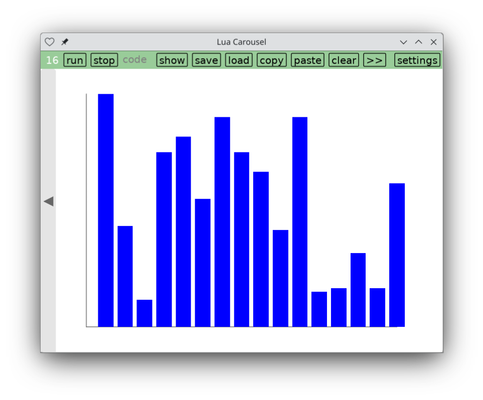
boxes, basically like single-type histograms:
plot(data, boxes, col(1), col(2))
boxerrorbars, which depends on a hack of using a transparent color:
color(0,0,1, 0.5)
plot(data, boxerrorbars, col(1), col(2), col(4))

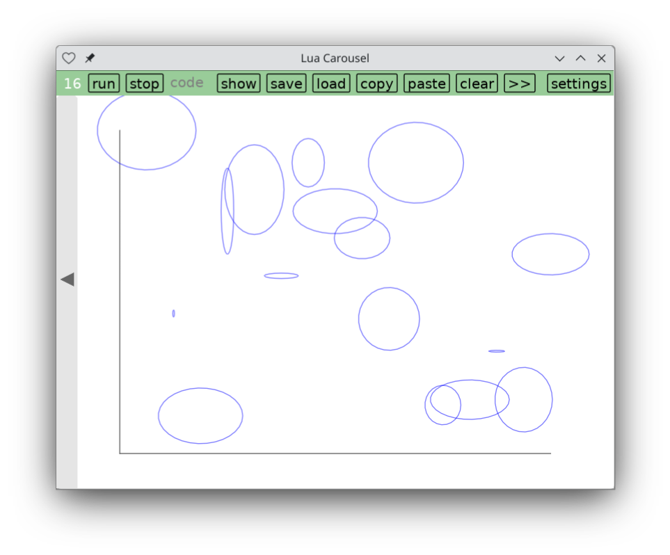
plot(data, ellipses, col(1), col(2), col(4), col(5), 'line')
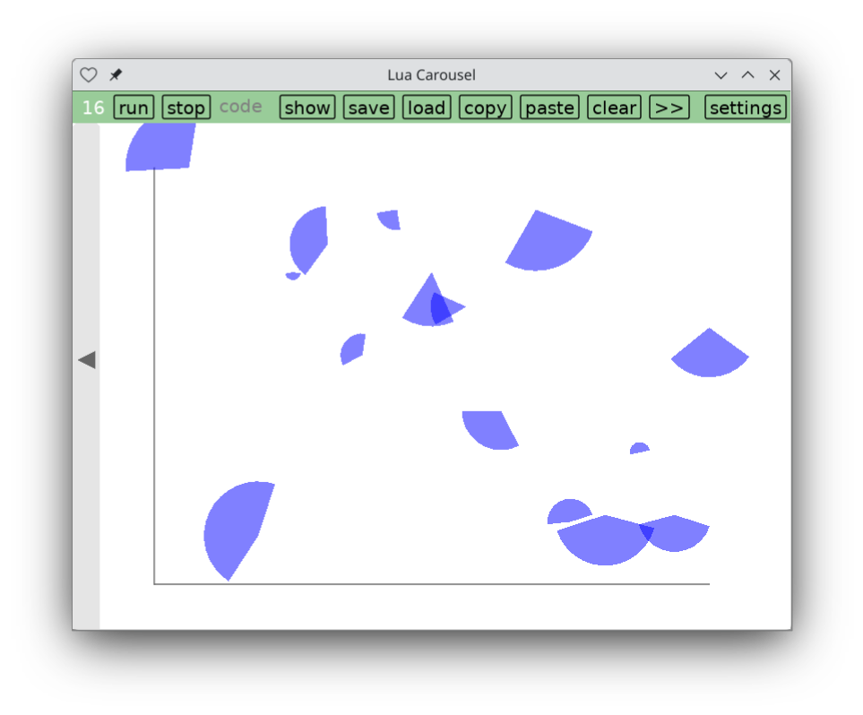
arcs, where we use our angle columns:
plot(data, arcs, col(1), col(2), col(4), col(6), col(7))
It turns out there's a whole variety of charts with error bars:
function xerrorbars(data, i, x, y, dx)
  local vy = vy(y(data, i))
  circle('fill', vx(x(data, i)), vy, 3)
  local x, dx = x(data, i), dx(data, i)
  line(vx(x-dx/2), vy, vx(x+dx/2), vy)
end
function xerrorlines(data, i, x, y, dx)
  do
    local vy = vy(y(data, i))
    circle('fill', vx(x(data, i)), vy, 3)
    local x, dx = x(data, i), dx(data, i)
    line(vx(x-dx/2), vy, vx(x+dx/2), vy)
  end
  if i == 1 then return end
  line(vx(x(data, i-1)), vy(y(data, i-1)), vx(x(data, i)), vy(y(data, i)))
end
function xerrorbars2(data, i, x, y, xlo, xhi)
  local vy = vy(y(data, i))
  circle('fill', vx(x(data, i)), vy, 3)
  line(vx(xlo(data, i)), vy, vx(xhi(data, i)), vy)
end
function xerrorlines2(data, i, x, y, xlo, xhi)
  do
    local vy = vy(y(data, i))
    circle('fill', vx(x(data, i)), vy, 3)
    line(vx(xlo(data, i)), vy, vx(xhi(data, i)), vy)
  end
  if i == 1 then return end
  line(vx(x(data, i-1)), vy(y(data, i-1)), vx(x(data, i)), vy(y(data, i)))
end
function yerrorbars(data, i, x, y, dy)
  local vx = vx(x(data, i))
  circle('fill', vx, vy(y(data, i)), 3)
  local y, dy = y(data, i), dy(data, i)
  line(vx, vy(y-dy/2), vx, vy(y+dy/2))
end
function yerrorlines(data, i, x, y, dy)
  do
    local vx = vx(x(data, i))
    circle('fill', vx, vy(y(data, i)), 3)
    local y, dy = y(data, i), dy(data, i)
    line(vx, vy(y-dy/2), vx, vy(y+dy/2))
  end
  if i == 1 then return end
  line(vx(x(data, i-1)), vy(y(data, i-1)), vx(x(data, i)), vy(y(data, i)))
end
function yerrorbars2(data, i, x, y, ylo, yhi)
  local vx = vx(x(data, i))
  circle('fill', vx, vy(y(data, i)), 3)
  line(vx, vy(ylo(data, i)), vx, vy(yhi(data, i)))
end
function yerrorlines2(data, i, x, y, ylo, yhi)
  do
    local vx = vx(x(data, i))
    circle('fill', vx, vy(y(data, i)), 3)
    line(vx, vy(ylo(data, i)), vx, vy(yhi(data, i)))
  end
  if i == 1 then return end
  line(vx(x(data, i-1)), vy(y(data, i-1)), vx(x(data, i)), vy(y(data, i)))
end
function xyerrorbars(data, i, x, y, dx, dy)
  local x, dx = x(data, i), dx(data, i)
  local y, dy = y(data, i), dy(data, i)
  circle('fill', vx(x), vy(y), 3)
  line(vx(x-dx/2), vy(y), vx(x+dx/2), vy(y))
  line(vx(x), vy(y-dy/2), vx(x), vy(y+dy/2))
end
function xyerrorlines(data, i, x, y, dx, dy)
  do
    local x, dx = x(data, i), dx(data, i)
    local y, dy = y(data, i), dy(data, i)
    circle('fill', vx(x), vy(y), 3)
    line(vx(x-dx/2), vy(y), vx(x+dx/2), vy(y))
    line(vx(x), vy(y-dy/2), vx(x), vy(y+dy/2))
  end
  if i == 1 then return end
  line(vx(x(data, i-1)), vy(y(data, i-1)), vx(x(data, i)), vy(y(data, i)))
end
function xyerrorbars2(data, i, x, y, xlo, xhi, ylo, yhi)
  circle('fill', vx(x), vy(y), 3)
  line(vx(xlo(data, i)), vy(y), vx(xhi(data, i)), vy(y))
  line(vx(x), vy(ylo(data, i)), vx(x), vy(yhi(data, i)))
end
function xyerrorlines2(data, i, x, y, xlo, xhi, ylo, yhi)
  circle('fill', vx(x), vy(y))
  line(vx(xlo(data, i)), vy(y), vx(xhi(data, i)), vy(y))
  line(vx(x), vy(ylo(data, i)), vx(x), vy(yhi(data, i)))
  if i == 1 then return end
  line(vx(x(data, i-1)), vy(y(data, i-1)), vx(x(data, i)), vy(y(data, i)))
end
function boxxyerror(data, i, x, y, dx, dy, drawmode)
  rect(optional(drawmode, data, i, 'line'), vx(x(data, i)), vy(y(data, i)), scale(dx(data, i)), scale(dy(data, i)))
end
function boxerrorbars(data, i, x, y, dy, w, drawmode)
  local w = optional(w, data, i, 4)
  local x = x(data, i)
  local y, dy = y(data, i), dy(data, i)
  rect(optional(drawmode, data, i, 'fill'), vx(x-w/2), vy(y), scale(w), vy(0) - vy(y))
  line(vx(x), vy(y-dy/2), vx(x), vy(y+dy/2))
end
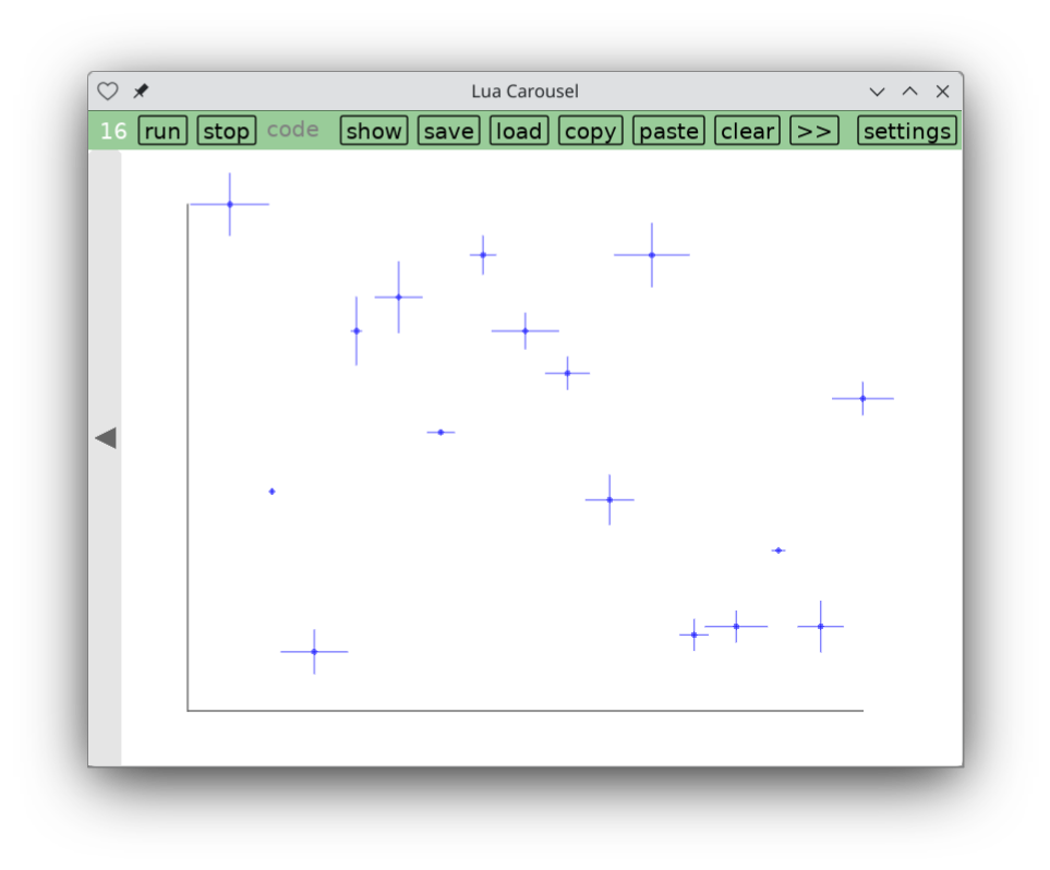
I'll just show one example from this set:
plot(data, xyerrorbars, col(1), col(2), col(4), col(5))
Alright, this post is getting long. Here's all the scaffolding code in one place:
-- decide how large a 80:60 image you can fit
H = Safe_height-Menu_bottom
if Safe_width/80 < H/60 then
  -- landscape
  v = {left=50, right=Safe_width-50}
  local h = (v.right-v.left)/80*60
  v.top = Menu_bottom + (H-h)/2
  v.bottom = v.top + h
else
  -- portrait
  v = {top=Menu_bottom+50, bottom=Safe_height-50}
  local w = (v.bottom-v.top)/60*80
  v.left = (Safe_width-w)/2
  v.right = v.left + w
end
-- at this point, 80/(v.right-v.left) == 60/(v.bottom-v.top)
line(v.left, v.top, v.left, v.bottom)
line(v.left, v.bottom, v.right, v.bottom)
function vx(x) return v.left + scale(x) end
function vy(y) return v.bottom - scale(y) end
function scale(d) return d/80*(v.right-v.left) end
function col(c)
  return function(data, i) return data[i][c] end
end
function plot(data, f, ...)
  for i=1,#data do f(data, i, ...) end
end
function optional(f, data, i, default)
  if f == nil then return default end
  if type(f) == 'function' then return f(data, i) end
  return f
end
This is the core. Paste it into a screen. Save my strategies above in a separate screen or two. Remember to first run the abbreviations on one of the example screens. Or if you've deleted that screen, here it is again:
-- Some abbreviations to reduce typing.
g = love.graphics
pt, line = g.points, g.line
rect, poly = g.rectangle, g.polygon
circle, arc, ellipse = g.circle, g.arc, g.ellipse
color = g.setColor
min, max = math.min, math.max
floor, ceil = math.floor, math.ceil
abs, rand = math.abs, math.random
pi, cos, sin = math.pi, math.cos, math.sin
touches = love.touch.getTouches
touch = love.touch.getPosition
audio = love.audio.newSource
Basically I keep a scratch screen around that looks like this:
run_screen('abbrev')
run_screen('plot')
run_screen('plots')
run_screen('errorplots')
data = {}
for i=1,16 do
  local angle1 = rand(60)/60*pi
  table.insert(data, {i*5, rand(60), rand(60), rand(60)/60*10, rand(60)/60*10, angle1, angle1+rand(60)/60*pi, tostring(rand(1000))})
end
color(0,0,1, 0.3)
plot(data, xyerrorbars, col(1), col(2), col(4), col(5))
Now I can replace `data` and the `plot` commands as needed. This seems to cover most of my needs, around half of gnuplot's subplot types. Of course, this is just for quick-and-dirty visualization, not publication-quality images. No support for 3D or heatmaps or polar coordinates. The next feature I want is histograms.
Leave a comment
Log in with itch.io to leave a comment.